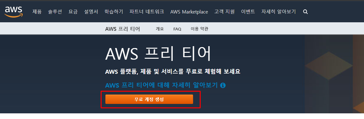
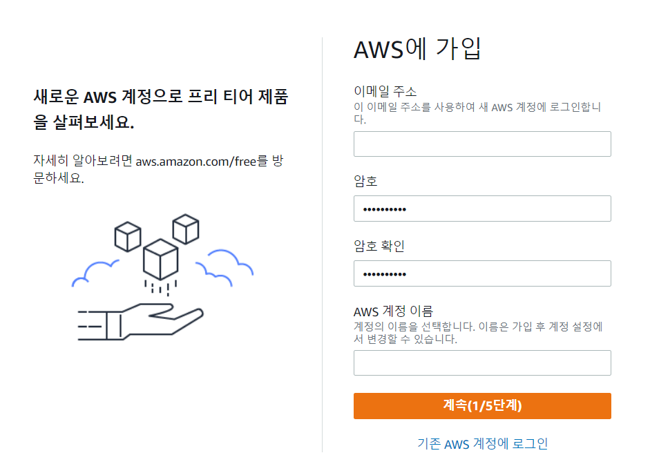
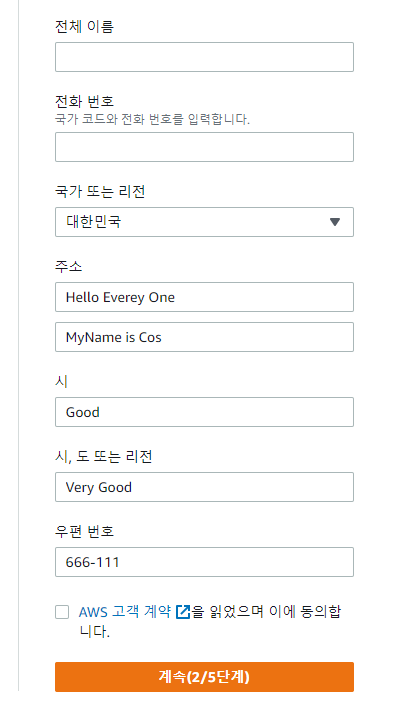
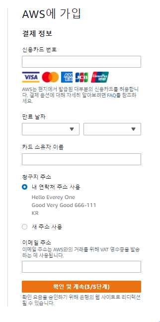
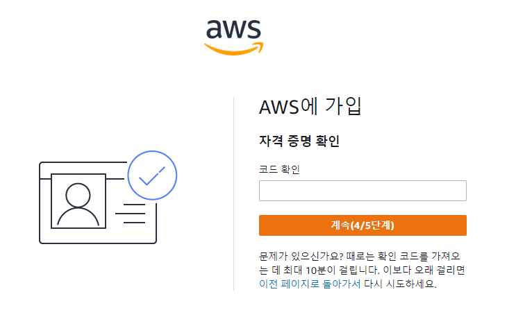
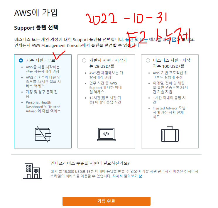
AWS 가입방법
무료 클라우드 컴퓨팅 서비스 - AWS 프리 티어
Internet Explorer에 대한 AWS 지원이 07/31/2022에 종료됩니다. 지원되는 브라우저는 Chrome, Firefox, Edge 및 Safari입니다. 자세히 알아보기
aws.amazon.com

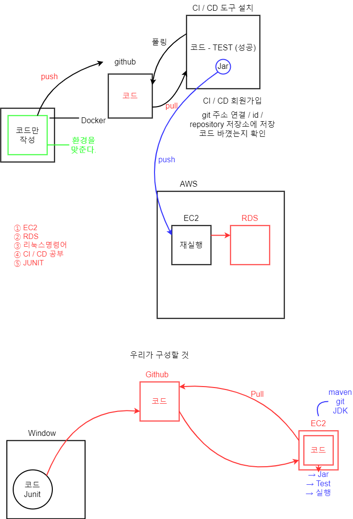
Docker / AWS 를 이용하여 프로젝트 실행할 예정!
도커 (소프트웨어) - 위키백과, 우리 모두의 백과사전
도커(Docker)는 리눅스의 응용 프로그램들을 프로세스 격리 기술들을 사용해 컨테이너로 실행하고 관리하는 오픈 소스 프로젝트이다. 도커 웹 페이지의 기능을 인용하면 다음과 같다: 도커 컨테
ko.wikipedia.org
https://raw.githubusercontent.com/rickiepark/hg-mldl/master/perch_full.csv
# 특성 공학과 규제

# 1. 데이터 준비
import pandas as pd
df = pd.read_csv("https://bit.ly/perch_csv_data") # read_csv : 파일, 웹 다 가능
perch_full = df.to_numpy()
print(perch_full)
농어의 길이와 무게 데이터
농어의 길이와 무게 데이터. GitHub Gist: instantly share code, notes, and snippets.
gist.github.com
import numpy as np

# https://bit.ly/perch_data
perch_weight = np.array([5.9, 32.0, 40.0, 51.5, 70.0, 100.0, 78.0, 80.0, 85.0, 85.0, 110.0,
       115.0, 125.0, 130.0, 120.0, 120.0, 130.0, 135.0, 110.0, 130.0,
       150.0, 145.0, 150.0, 170.0, 225.0, 145.0, 188.0, 180.0, 197.0,
       218.0, 300.0, 260.0, 265.0, 250.0, 250.0, 300.0, 320.0, 514.0,
       556.0, 840.0, 685.0, 700.0, 700.0, 690.0, 900.0, 650.0, 820.0,
       850.0, 900.0, 1015.0, 820.0, 1100.0, 1000.0, 1100.0, 1000.0,
       1000.0])

from sklearn.model_selection import train_test_split
train_input, test_input, train_target, test_target = train_test_split(
    perch_full, perch_weight, random_state = 42
)
from sklearn.preprocessing import PolynomialFeatures
poly = PolynomialFeatures(include_bias=False)
# fit을 해야 transform이 가능하다. x, y, x^2, y^2, x*y
# 훈련을 해야 변환이 가능하다.
poly.fit([[2,5]])
print(poly.transform([[2,5]]))
poly.fit(train_input) # 길이, 높이 두께
train_poly = poly.transform(train_input)
test_poly = poly.transform(test_input)
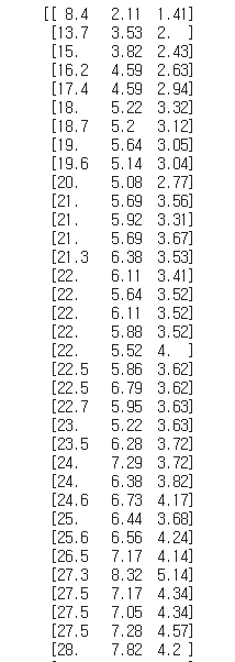
print(train_poly[:3])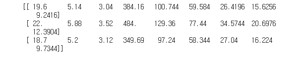
poly.get_feature_names()
from sklearn.linear_model import LinearRegression
lr = LinearRegression()
lr.fit(train_poly, train_target)
print(lr.score(train_poly, train_target))
print(lr.score(test_poly, test_target))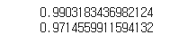
- 다중회귀 : 여러 개의 특성을 사용한 선형 회귀
- 특성공학 : 기존의 특성을 사용해 새로운 특성을 뽑아내는 작업
# 다중 특성이나 다항이나 결국(특성을 늘리는 것(더미데이터))
# → PolynomialFeatures 라이브러리를 사용하면 특성을 쉽게 늘릴 수 있다.
# → 너무 훈련에 적합해질 수 있다. → 규제

# x좌표 1~100. y좌표 100~1000
# 분산 → 표준편차 std() → 표준점수 (원래값 - 예측값) / std → 표준점수 [1,3,5] - 3 / 표준편차
# → StandardScaler 라이브러리를 사용하면 스케일링을 쉽게 할 수 있다.

from sklearn.preprocessing import StandardScaler
ss = StandardScaler()
# 스케일링 하기
ss.fit(train_poly)
train_scaled = ss.transform(train_poly)
test_scaled = ss.transform(test_poly)

# 어떤 2차원 데이터가 있음 → 특징을 찾아내기 → 분류, (회귀) → cross-validation → 선형회귀 훈련
# 스케일링(x,y의 수치 차이) and 특성을 강제로 늘리기(더미)
print(train_poly[:3])
print(train_scaled[:3])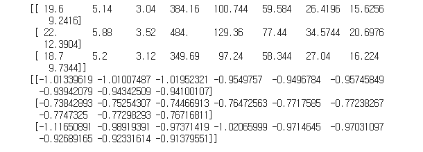
from sklearn.linear_model import Ridge
ridge = Ridge(alpha=3)  # alpha

ridge.fit(train_scaled, train_target)
print(ridge.score(train_scaled,train_target))
print(ridge.score(test_scaled,test_target))

# 원본
# 0.9903183436982124
# 0.9714559911594132

# 규제
# 0.9857915060511934
# 0.9835057194929057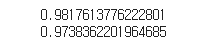
import matplotlib.pyplot as plt

plt.plot(train_scaled, train_target)
plt.show()

print(train_target)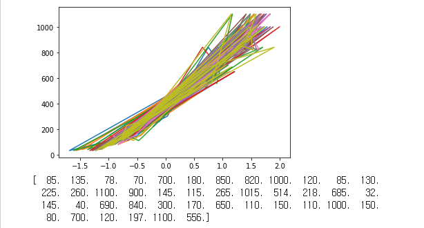
a = 16 # 2의 4승

b = np.log2(a)
print(b)

# 로그 → 엄청나게 큰 수를 작은 수로 표현할 수 있다.

c = 32
d = np.log(c) # e → 자연상수 2.71797~~~~~~~~~
print(d)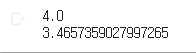
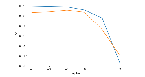
# 최적의 alpha값 찾아보기
import matplotlib.pyplot as plt
train_score = []
test_score = []
alpha_list = [0.001, 0.01, 0.1, 1, 10, 100]
for alpha in alpha_list:
  ridge = Ridge(alpha=alpha)
  ridge.fit(train_scaled, train_target)
  train_score.append(ridge.score(train_scaled, train_target))
  test_score.append(ridge.score(test_scaled, test_target))
# 로그를 이용해서 값을 지수로 표현하기
plt.plot(np.log10(alpha_list), train_score)
plt.plot(np.log10(alpha_list), test_score)
plt.xlabel("alpha")
plt.ylabel("R^2")
plt.show()
'Programming > Machine Learning' 카테고리의 다른 글
| Machine Leaning 3 - 1강 - 결정 계수 , 과소 • 과대 적합 , 경사 하강법 (0) | 2021.10.28 |
|---|---|
| Machine Leaning 2-2강 - 분산, 표준편차, 오차율, 회귀, 표준점수 (0) | 2021.10.27 |
| Machine Leaning 2-1강 - split , shuffle, index (0) | 2021.10.27 |
| Machine Learning 1강 - 최근접 이웃(KNeighborsClassifier) (0) | 2021.10.27 |